


Are the Best Athletes the Most Likely to Choke under Pressure?
The correct conclusion Alex Hutchinson should have drawn in "Why Performance Under Pressure Isn't All in Your Head"

I greatly enjoyed and highly recommend Alex Hutchinson’s most recent book Endure. This led me to his Outside magazine “Sweat Science” column. Plenty of good reading, but occasionally Alex draws the wrong conclusion due to not catching statistical methodology errors in the research he draws on.
Statistical Rethinking by Richard McElreath, also available as a video lecture series is a general remedy for gaining sufficient mastery to spot statistics mistakes. Prof. McElreath is currently delivering an updated (2022) video lecture series, which likely has improved content and efficiency. But the 2019 series is more entertaining — more jokes! — since he’s presenting to an actual classroom.
For now, I’ll cover two errors I noticed in Alex’s 3/2/22 article “Why Performance Under Pressure Isn’t All in Your Head”.
Alex accepts the finding from “An Analysis of Playoff Performance Declines in Major League Baseball” (Conforti, Crotin & Oseguera — henceforth, ‘CC&O’ — Journal of Strength and Condition Research, 12/1/22) that baseball players (1) generally perform worse in the playoffs (2) with the best players suffering the greatest decline.
These findings are not supported by the data.
By using raw regular season results as their benchmark for evaluating playoff performance, CC&O omit two vital adjustments:
Playoff opponents are, on average, better than regular season opponents
Statistical regression toward the mean
CC&O used advanced metrics data for 1477 MLB players from 1994 to 2019 publicly available at Fangraphs — Fielding Independent Pitching (FIP), Weighted Runs Created Plus (wRC+) and Errors per Inning Out (EpIO) — to evaluate, respectively, pitching, hitting and defensive performance. They partitioned the athletes into quartiles for each of these three skills.
For pitching and hitting, CC&O obtained the results noted above: all quartiles did worse in the playoffs, and the magnitude of decline increased from the lowest to highest quartile. In fielding, the top two quartiles did worse, but both lower quartiles did better.
The reason for the general decline is that players on teams that make the playoffs tend to be better than average. As a result, playoff pitchers must face better hitters than they did during the regular season; similarly, the playoff batters have to face better pitchers. One way to adjust for this altered environment would be to limit the regular season data to games against playoff teams; further refinements in this direction can be made.
In contrast, fielding errors are a (nearly) solo responsibility, which can be fully accounted for by regression toward the mean. Regression toward the mean (and not, say, choking) also produces the increased decline for better regular season performers.
To explain statistical regression toward the mean, here’s an example from my childhood. Rico Carty of the Atlanta Braves started the 1970 season red hot. At the end of April, he was batting .423 (33 hits in 78 at bats). Could he bat .400 for the season?
An introductory statistics course might lead you to believe he was more likely than not since (in Stats 101) you learn that the average is an ‘unbiased estimator’ of the probability that in any given at bat, Carty would get a hit.
But just because an estimator is unbiased, it may not be perfectly accurate. In fact, suitably biased estimators invariably produce more accurate predictions!
Bayesian Statistics provides a systematic way to acknowledge the fact that Rico’s end-of-April batting average was not a precise measurement of his probability of getting a hit in each at bat.
Start with a prior distribution that reflects our uncertainty about this probability. Then update this prior using the data we’ve collected, i.e., use Bayes’ rule, to compute a posterior distribution. This posterior will be a better assessment of Rico’s probability of getting a hit than either the prior or his actual batting average. As a result, it will make a more accurate prediction of his batting average for the rest of the season.
For binomial data — that is, the outcome of each trial is either success or failure — the beta distribution is a natural prior. For 1970 MLB batting, I estimated beta distribution parameters α=20, β=59.1 With these parameters, the beta distribution has a mean value of α/(α+β)= 0.253 and a variance of αβ/((α+β)^2(α+β+1)), corresponding to a standard deviation of about 0.049.
The information encapsulated in this prior is that the average ability of 1970’s hitters is to bat .253 … but they don’t all have the identical expectation of a 25.3% chance of getting a hit in any given at bat. Instead, for example, about 16% of the hitters expect to get a hit 30% of the time or more (the beta distribution is approximately a normal distribution, so about 1/6th of this distribution lies at least one standard deviation above the average).
At the end of April, update this prior distribution by adding the number of successes (Rico’s hits) to α — α'=20+33=53 — and the number of failures (Rico’s outs) to β — β'=59+45=104.2 So our posterior distribution for Rico’s expected batting average based on April is Beta(53,104). The mean value of this posterior is α'/(α'+β')=.338; the standard deviation is .038. That’s our (biased) prediction of Rico’s batting average for the rest of the 1970 season.3
Rico made things even more exciting with a scorching May, closing the month at .436 (72 for 165). All in all, he batted .355 (142 for 400) after April, for a season total batting average of .366.
It may be intuitively obvious that .338 (our biased estimate) is a better prediction than .423 (the unbiased estimate) for Rico’s batting average for the remainder of the 1970 season. To firm up that intuition, consider what we learn from Rico’s performance in April. Sure, a league average .250 hitter could get really lucky and bat .423 for a month. But it’s more likely that Rico is a (much) better than average hitter. How much better? Well, it’s still unlikely that Rico (or anyone else in the league) can actually expect to get a hit 42% of the time (that’s more than three standard deviations above average). Instead, the most likely way to produce 33 hits in 78 bats is to combine great skill with good luck. Bayes’ rule accurately blends these possibilities into the posterior distribution.
More generally, regular season baseball performance gives us useful information about the players’ skills. But to accurately project playoff performance, we shouldn’t take the regular season results as perfect measurements of the players’ abilities. We need to accurately acknowledge the luck component: a mediocre player can be really lucky and have a great season, while an unlucky but great player might have a run-of-the-mill summer.
Combining reasonable prior distributions with the regular season results will improve our playoff predictions. When we do this, we’ll expect to see something that’s often termed ‘regression to the mean’. But it’s not regression all the way to the mean; it’s better described as ‘regression toward the mean’.
Unless we’re predicting a skill-free activity, above average performances are indicative of above average skill. But they’re also indicative of good luck, and Bayes’ rule tells us exactly how to balance these two indications.
To summarize: to assess how players respond to pressure you must benchmark against an accurate prediction of that performance (in the absence of pressure), rather than just comparing against ‘raw’ regular season performance.
CC&O’s conclusion …
teams should consider providing greater mental performance support, implement periodization strategies to taper or lower training workloads, offer team support networks, and anxiety desensitization for excellent MLB performers in approach of the playoffs, as certain aspects of pitching and hitting significantly suffer.
… is completely unsupported at this time. It’s still possible that the best athletes are more likely to choke or burn out. But before we draw that conclusion, we must (1) adjust for playing conditions and (2) measure skill accurately.
The second of these requires some statistical savvy because in any stochastic activity, skill is not directly observable. Instead we have to infer an athlete’s skill by using the actual outcomes to update the prior knowledge that we have acquired.
Technical postscript
To get an idea of what degree of regression toward the mean to expect when comparing regular season baseball data to the playoffs, here’s a ‘lite’ replication of CC&O’s study. To reduce my workload, I just looked at the 2021 season. I’m not sure why, but I wasn’t able to get 2021 postseason data from Fangraphs. So I instead used results from April through August to predict performance from September through October 3 (the end of the regular season). Also, because I wanted to easily apply Bayes’ rule, I evaluated OBP (on base percentage). Each plate appearance can be viewed as a binomial trial; the advanced metrics CC&O examined are interval scale random variables with more complicated distributions.
Despite these study design differences, the results are similar. The best ‘early’ batters exhibited the greatest declines at the end of the regular season.

From the slope of regression line, we see that there is about a 45% (=1-0.5494) regression toward the mean.
My estimates of the beta distribution parameters for getting on base in 2021: α=24, β=50. The expected regression toward the mean is (α+β)/(n+α+β), where n is the number of plate appearances observed (in the first part of the season).
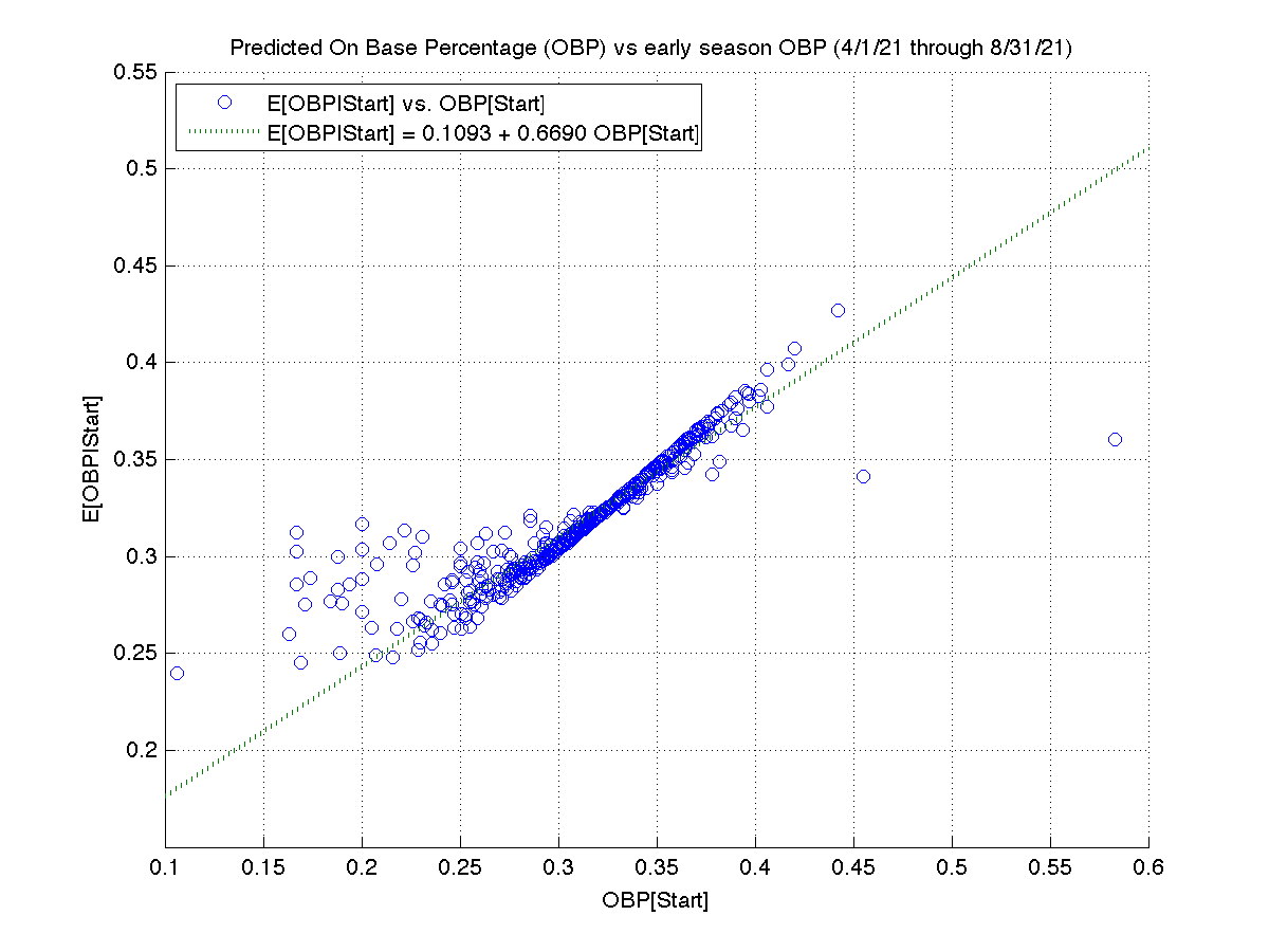
My Bayesian model predicts an average mean reversion of about 31% (1 - 0.6690), accounting for (only) about two-thirds of the mean reversion we actually observe. The biggest reason for this shortfall is non-stationarity: batters don’t have an identical probability of getting on base in each plate appearance. For example, the pitchers they face vary in quality; some parks have large foul territories (allowing fielders to catch more foul popups). The most important contribution to non-stationarity is that hitters have hot and cold streaks. The cold streaks are typically due to injury and fatigue.
Augmenting the predictive model for non-stationarity is much more involved, so I’ll leave that for a future report.
In a possible future report, I could explain how I estimated these parameter values.
In that future report, I could discuss how conjugate priors simplify the application of Bayes’ Rule.
The unbiased estimator is

and the standard error of this unbiased estimator is

This is almost 50% larger than the standard deviation of our posterior estimate. From the perspective of variance, our biased estimate — .338(.038) — is more than twice as accurate as the unbiased estimate — 0.423(.056).